BerlinMOD Example

This example uses synthetic trip data in Brussels generated by the MobilityDB-BerlinMOD generator to show some data manipulations available in PyMEOS. It is divided in 5 sections, each corresponding to one MEOS example:

• Disassembling Trips

• Clipping Trips to Geometries

• Tiling Trips

• Simplifying Trips

• Temporal Aggregation of Trips

This example uses the plotting capabilities of PyMEOS. To get the necessary dependencies for this example, you can run the following command:

pip install pymeos[plot, pandas] contextily distinctipy

from datetime import timedelta
from functools import partial

import contextily as cx
import distinctipy
import geopandas as gpd
import matplotlib.pyplot as plt
import pandas as pd
import shapely.geometry as shp
from pymeos import *
from pymeos.plotters import (
    TemporalPointSequenceSetPlotter,
    TemporalPointSequencePlotter,
)
from shapely import wkb

pymeos_initialize()

In every following section we use the data from the BerlinMOD Generator, so we will go ahead and read it.

trips = pd.read_csv(
    "./data/trips.csv",
    converters={
        "trip": TGeomPointSeq,
    },
)
trips.head()

	vehicle	day	seq	trip
0	1	2020-06-01	1	[POINT(496253.84080706234 6601691.244869352)@2...
1	1	2020-06-01	2	[POINT(481241.17182724166 6588272.126511315)@2...
2	1	2020-06-02	1	[POINT(496253.84080706234 6601691.244869352)@2...
3	1	2020-06-02	2	[POINT(481241.17182724166 6588272.126511315)@2...
4	1	2020-06-03	1	[POINT(496253.84080706234 6601691.244869352)@2...

Disassembling Trips (MEOS Example)

In this section, we disassemble the trips into individual observations and write them in a CSV file ordered by timestamp.

First, we’ll obtain every timestamp and value from the trajectory object (TGeogPointSeq) using the timestamps and values functions respectively

records = trips.drop("trip", axis=1).copy()
records["geom"] = trips["trip"].apply(lambda tr: tr.values())
records["t"] = trips["trip"].apply(lambda tr: tr.timestamps())
records.head()

	vehicle	day	seq	geom	t
0	1	2020-06-01	1	[POINT (496253.84080706234 6601691.244869352),...	[2020-06-01 11:48:50.886000+02:00, 2020-06-01 ...
1	1	2020-06-01	2	[POINT (481241.17182724166 6588272.126511315),...	[2020-06-01 18:00:27.208000+02:00, 2020-06-01 ...
2	1	2020-06-02	1	[POINT (496253.84080706234 6601691.244869352),...	[2020-06-02 11:31:07.888000+02:00, 2020-06-02 ...
3	1	2020-06-02	2	[POINT (481241.17182724166 6588272.126511315),...	[2020-06-02 18:47:26.738000+02:00, 2020-06-02 ...
4	1	2020-06-03	1	[POINT (496253.84080706234 6601691.244869352),...	[2020-06-03 11:30:29.334000+02:00, 2020-06-03 ...

Now we “explode” the t and geom columns to get a row per record. Then, we sort the records by timestamp.

records = records.explode(["geom", "t"], ignore_index=True)
records = records.sort_values("t")
records.head()

	vehicle	day	seq	geom	t
110254	8	2020-06-01	1	POINT (493442.7231019071 6595901.46838472)	2020-06-01 10:22:51.025000+02:00
110255	8	2020-06-01	1	POINT (493443.8028284878 6595906.350412016)	2020-06-01 10:22:52.525000+02:00
110256	8	2020-06-01	1	POINT (493444.404026218 6595909.068751807)	2020-06-01 10:22:54.574117+02:00
110257	8	2020-06-01	1	POINT (493441.7878750556 6595913.329708636)	2020-06-01 10:22:55.639765+02:00
110258	8	2020-06-01	1	POINT (493428.7071192439 6595934.634492779)	2020-06-01 10:23:00.139765+02:00

Finally, we will write it in a CSV file, encoding first the geometries as HexWKB

records["geom"] = records["geom"].apply(partial(wkb.dumps, hex=True))
records.head()

	vehicle	day	seq	geom	t
110254	8	2020-06-01	1	01010000008BD374E40A1E1E41E803FA5D4F295941	2020-06-01 10:22:51.025000+02:00
110255	8	2020-06-01	1	0101000000CEAB18360F1E1E4185266D9650295941	2020-06-01 10:22:52.525000+02:00
110256	8	2020-06-01	1	0101000000840CB99D111E1E41FB6D664451295941	2020-06-01 10:22:54.574117+02:00
110257	8	2020-06-01	1	0101000000F5B7C826071E1E4140F2195552295941	2020-06-01 10:22:55.639765+02:00
110258	8	2020-06-01	1	01010000002C1117D4D21D1E419A879BA857295941	2020-06-01 10:23:00.139765+02:00

records.to_csv("./data/trip_instants.csv", index=False)

Clipping Trips to Geometries (MEOS Example)

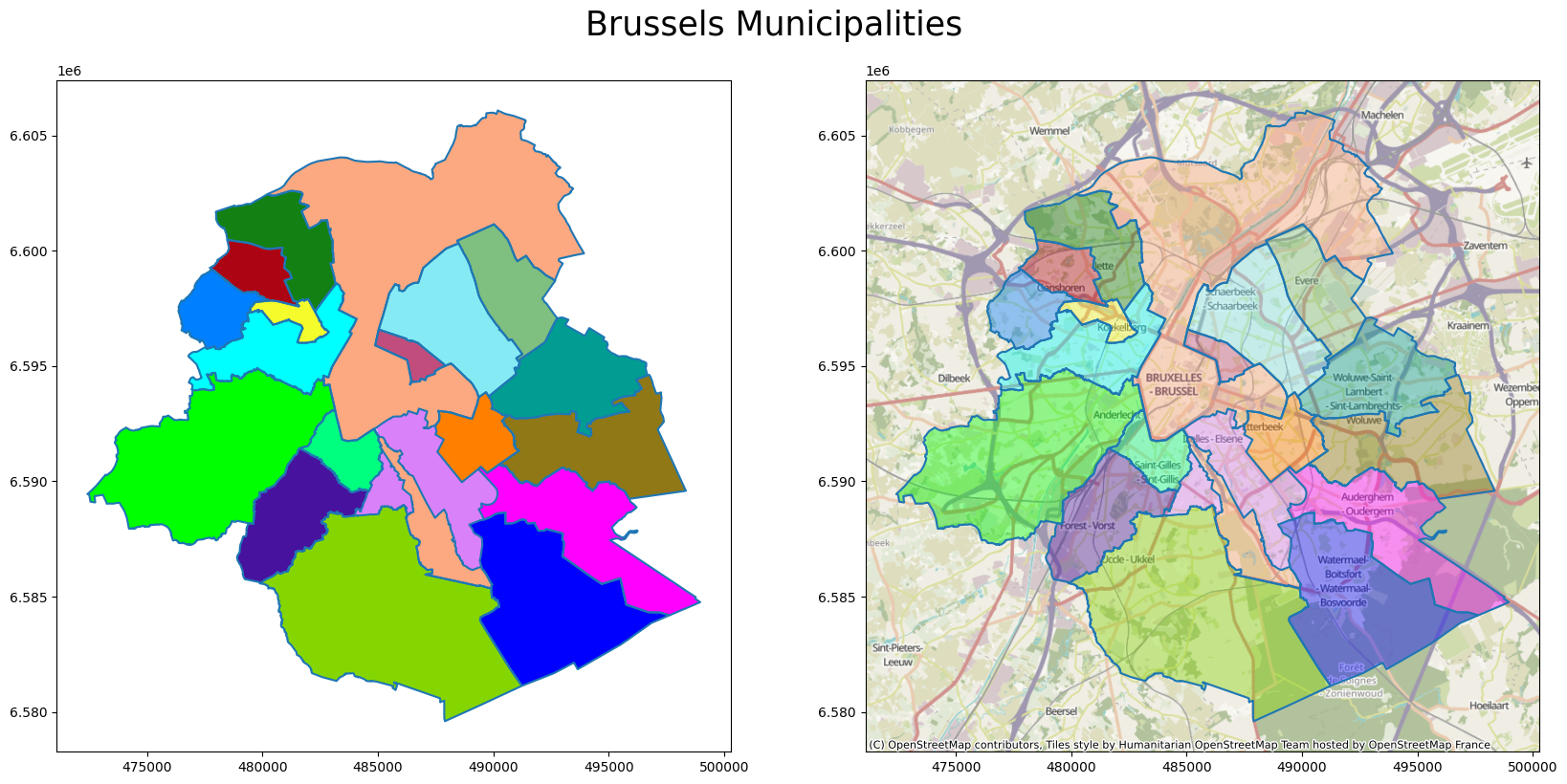
In this section, we compute the distance traversed by the trips in the 19 Brussels municipalities (communes in French)

First, we will read the files containing the information about the Brussels region and its municipalities and take a look at their shape

brussels = pd.read_csv(
    "./data/brussels_region.csv", converters={"geom": partial(wkb.loads, hex=True)}
)
brussels = gpd.GeoDataFrame(brussels, geometry="geom")
brussels_geom = brussels["geom"][0]
brussels

	name	geom
0	Région de Bruxelles-Capitale - Brussels Hoofds...	POLYGON ((472413.848 6589441.686, 472482.354 6...

communes = pd.read_csv(
    "./data/communes.csv", converters={"geom": partial(wkb.loads, hex=True)}
)
communes["color"] = [
    "#00ff00",
    "#ff00ff",
    "#007fff",
    "#ff7f00",
    "#7fbf7f",
    "#47139e",
    "#ad0414",
    "#d981f9",
    "#138014",
    "#f4fc2c",
    "#00ffff",
    "#00ff7f",
    "#c04d7c",
    "#85eaf3",
    "#85d601",
    "#fca880",
    "#0000ff",
    "#019d92",
    "#907817",
]
communes = gpd.GeoDataFrame(communes, geometry="geom")
communes

	id	name	population	geom	color
0	1	Anderlecht	118241	POLYGON ((476959.746 6593981.357, 476965.401 6...	#00ff00
1	2	Auderghem - Oudergem	33313	POLYGON ((497620.844 6584185.646, 497856.652 6...	#ff00ff
2	3	Berchem-Sainte-Agathe - Sint-Agatha-Berchem	24701	POLYGON ((477788.720 6599192.996, 477782.631 6...	#007fff
3	4	Etterbeek	176545	POLYGON ((489804.602 6593678.230, 489685.067 6...	#ff7f00
4	5	Evere	47414	POLYGON ((492771.667 6597070.173, 492633.519 6...	#7fbf7f
5	6	Forest - Vorst	40394	POLYGON ((479909.268 6585570.952, 479881.003 6...	#47139e
6	7	Ganshoren	55746	POLYGON ((478477.209 6600450.089, 478499.863 6...	#ad0414
7	8	Ixelles - Elsene	24596	MULTIPOLYGON (((487496.626 6592340.790, 487544...	#d981f9
8	9	Jette	86244	POLYGON ((481479.217 6597749.534, 481526.350 6...	#138014
9	10	Koekelberg	51933	POLYGON ((480236.024 6597825.520, 480178.160 6...	#f4fc2c
10	11	Molenbeek-Saint-Jean - Sint-Jans-Molenbeek	21609	POLYGON ((477542.960 6595837.350, 477533.621 6...	#00ffff
11	12	Saint-Gilles - Sint-Gillis	96629	POLYGON ((483153.140 6593066.827, 483122.204 6...	#00ff7f
12	13	Saint-Josse-ten-Noode - Sint-Joost-ten-Node	50471	POLYGON ((485033.738 6596581.156, 484882.700 6...	#c04d7c
13	14	Schaerbeek - Schaarbeek	27115	POLYGON ((488501.707 6600305.815, 488394.028 6...	#85eaf3
14	15	Uccle - Ukkel	133042	POLYGON ((486268.683 6588562.809, 486253.744 6...	#85d601
15	16	Ville de Bruxelles - Stad Brussel	82307	POLYGON ((483153.140 6593066.827, 483186.758 6...	#fca880
16	17	Watermael-Boitsfort - Watermaal-Bosvoorde	24871	POLYGON ((491240.935 6581131.551, 491340.822 6...	#0000ff
17	18	Woluwe-Saint-Lambert - Sint-Lambrechts-Woluwe	55216	POLYGON ((496682.744 6594589.884, 496653.033 6...	#019d92
18	19	Woluwe-Saint-Pierre - Sint-Pieters-Woluwe	41217	POLYGON ((496135.453 6589271.827, 496258.928 6...	#907817

_, axes = plt.subplots(1, 2, figsize=(20, 10))
communes.plot(color=communes["color"], ax=axes[0])
communes.exterior.plot(ax=axes[0])
communes.plot(color=communes["color"], ax=axes[1], alpha=0.4)
communes.exterior.plot(ax=axes[1])
cx.add_basemap(axes[1])
_ = plt.suptitle("Brussels Municipalities", size=25, y=0.92)

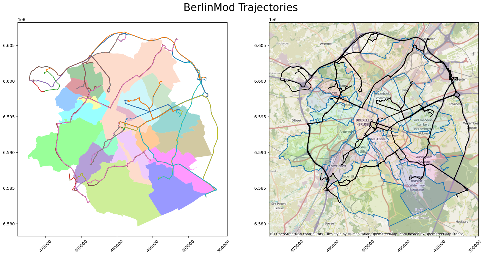
Now, let’s take a look at the BerlinMOD trajectories plotted over Brussels

_, axes = plt.subplots(1, 2, figsize=(20, 10))
communes.plot(color=communes["color"], ax=axes[0], alpha=0.4)

TemporalPointSequencePlotter.plot_sequences_xy(
    trips["trip"], axes=axes[0], show_markers=False, show_grid=False
)

communes.plot(color=communes["color"], ax=axes[1], alpha=0.1)
communes.exterior.plot(ax=axes[1])
TemporalPointSequencePlotter.plot_sequences_xy(
    trips["trip"], axes=axes[1], color="black", show_markers=False, show_grid=False
)
cx.add_basemap(axes[1])

_ = plt.suptitle("BerlinMod Trajectories", size=25, y=0.92)

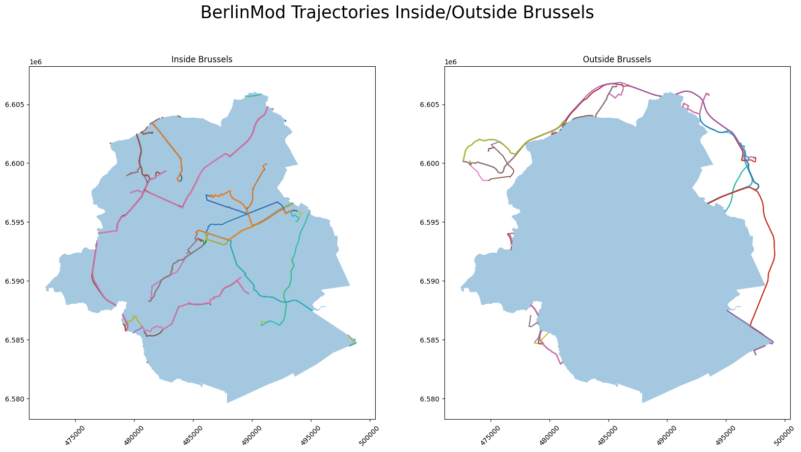
First, let’s split the trajectories into sections inside and outside of Brussels

brussels_inout_trajectories = trips.copy()
brussels_inout_trajectories["inside"] = brussels_inout_trajectories["trip"].apply(
    lambda tr: tr.at(brussels_geom)
)
brussels_inout_trajectories["outside"] = brussels_inout_trajectories["trip"].apply(
    lambda tr: tr.minus(brussels_geom)
)
brussels_inout_trajectories.head()

	vehicle	day	seq	trip	inside	outside
0	1	2020-06-01	1	[POINT(496253.84080706234 6601691.244869352)@2...	{[POINT(493452.04564533016 6596592.507628961)@...	{[POINT(496253.84080706234 6601691.244869352)@...
1	1	2020-06-01	2	[POINT(481241.17182724166 6588272.126511315)@2...	{[POINT(481241.17182724166 6588272.126511315)@...	{(POINT(493488.118266309 6596572.0201423885)@2...
2	1	2020-06-02	1	[POINT(496253.84080706234 6601691.244869352)@2...	{[POINT(493452.04567213746 6596592.507642428)@...	{[POINT(496253.84080706234 6601691.244869352)@...
3	1	2020-06-02	2	[POINT(481241.17182724166 6588272.126511315)@2...	{[POINT(481241.17182724166 6588272.126511315)@...	{(POINT(493488.118266309 6596572.0201423885)@2...
4	1	2020-06-03	1	[POINT(496253.84080706234 6601691.244869352)@2...	{[POINT(493452.04567213746 6596592.507642428)@...	{[POINT(496253.84080706234 6601691.244869352)@...

Let’s see this split in a plot

_, axes = plt.subplots(1, 2, figsize=(20, 10))

axes[0].set_title("Inside Brussels")
brussels.plot(ax=axes[0], alpha=0.4)
for traj in brussels_inout_trajectories["inside"].dropna():
    if isinstance(traj, TGeomPointSeq):
        TemporalPointSequencePlotter.plot_xy(
            traj, axes=axes[0], show_markers=False, show_grid=False
        )
    else:
        TemporalPointSequenceSetPlotter.plot_xy(
            traj, axes=axes[0], show_markers=False, show_grid=False
        )

axes[1].set_title("Outside Brussels")
brussels.plot(ax=axes[1], alpha=0.4)
for traj in brussels_inout_trajectories["outside"].dropna():
    if isinstance(traj, TGeomPointSeq):
        TemporalPointSequencePlotter.plot_xy(
            traj, axes=axes[1], show_markers=False, show_grid=False
        )
    else:
        TemporalPointSequenceSetPlotter.plot_xy(
            traj, axes=axes[1], show_markers=False, show_grid=False
        )

axes[0].set_xlim(
    min(axes[0].get_xlim()[0], axes[1].get_xlim()[0]),
    max(axes[0].get_xlim()[1], axes[1].get_xlim()[1]),
)
axes[0].set_ylim(
    min(axes[0].get_ylim()[0], axes[1].get_ylim()[0]),
    max(axes[0].get_ylim()[1], axes[1].get_ylim()[1]),
)

_ = plt.suptitle("BerlinMod Trajectories Inside/Outside Brussels", size=25)

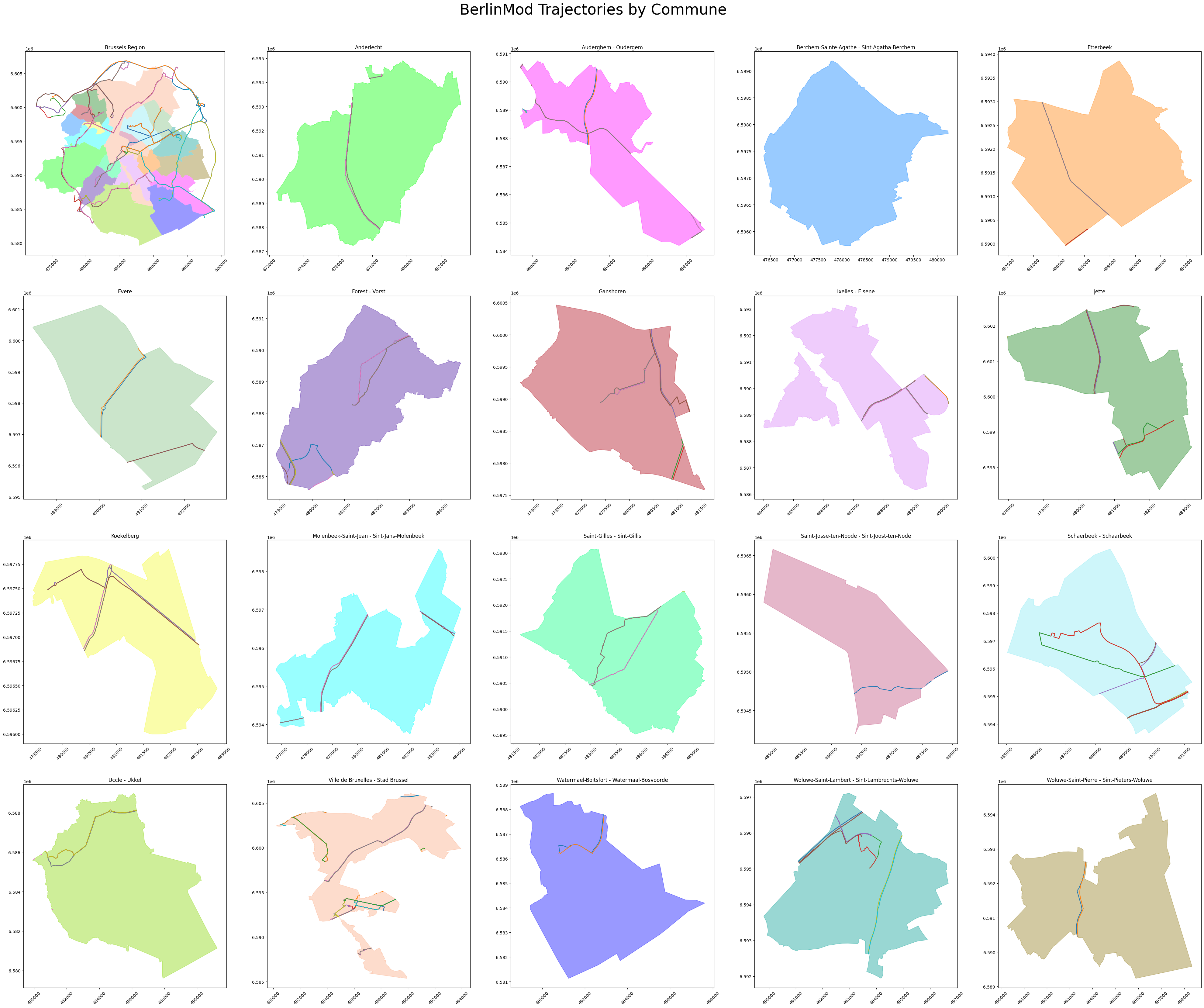
Now we will compute the trajectory and distance each trip traverses in each municipality

commune_trajectories = trips.copy()
for _, row in communes.iterrows():
    commune_trajectories[f'{row["name"]}-trajectory'] = commune_trajectories[
        "trip"
    ].apply(lambda tr: tr.at(row["geom"]))
    commune_trajectories[f'{row["name"]}-distance'] = commune_trajectories[
        f'{row["name"]}-trajectory'
    ].apply(lambda tr: tr.length() if tr else 0)
commune_trajectories.head()

	vehicle	day	seq	trip	Anderlecht-trajectory	Anderlecht-distance	Auderghem - Oudergem-trajectory	Auderghem - Oudergem-distance	Berchem-Sainte-Agathe - Sint-Agatha-Berchem-trajectory	Berchem-Sainte-Agathe - Sint-Agatha-Berchem-distance	...	Uccle - Ukkel-trajectory	Uccle - Ukkel-distance	Ville de Bruxelles - Stad Brussel-trajectory	Ville de Bruxelles - Stad Brussel-distance	Watermael-Boitsfort - Watermaal-Bosvoorde-trajectory	Watermael-Boitsfort - Watermaal-Bosvoorde-distance	Woluwe-Saint-Lambert - Sint-Lambrechts-Woluwe-trajectory	Woluwe-Saint-Lambert - Sint-Lambrechts-Woluwe-distance	Woluwe-Saint-Pierre - Sint-Pieters-Woluwe-trajectory	Woluwe-Saint-Pierre - Sint-Pieters-Woluwe-distance
0	1	2020-06-01	1	[POINT(496253.84080706234 6601691.244869352)@2...	None	0.0	None	0.0	None	0	...	None	0.0	{[POINT(489089.14461377583 6594225.227862967)@...	6238.532446	None	0.0	{[POINT(493452.04564533016 6596592.507628961)@...	2743.319101	None	0.0
1	1	2020-06-01	2	[POINT(481241.17182724166 6588272.126511315)@2...	None	0.0	None	0.0	None	0	...	None	0.0	{[POINT(484373.02614611824 6591974.073148593)@...	5890.625638	None	0.0	{[POINT(491131.62956994347 6595158.952745219)@...	2753.083663	None	0.0
2	1	2020-06-02	1	[POINT(496253.84080706234 6601691.244869352)@2...	None	0.0	None	0.0	None	0	...	None	0.0	{[POINT(489089.14461377583 6594225.227862967)@...	6238.532450	None	0.0	{[POINT(493452.04567213746 6596592.507642428)@...	2743.319131	None	0.0
3	1	2020-06-02	2	[POINT(481241.17182724166 6588272.126511315)@2...	None	0.0	None	0.0	None	0	...	None	0.0	{[POINT(484373.02614611824 6591974.073148593)@...	5890.625638	None	0.0	{[POINT(491131.62956994347 6595158.952745219)@...	2753.083663	None	0.0
4	1	2020-06-03	1	[POINT(496253.84080706234 6601691.244869352)@2...	None	0.0	None	0.0	None	0	...	None	0.0	{[POINT(489089.14461377583 6594225.227862967)@...	6238.532450	None	0.0	{[POINT(493452.04567213746 6596592.507642428)@...	2743.319131	None	0.0

5 rows × 42 columns

distances = commune_trajectories[
    ["vehicle", "day", "seq", *(f"{commune}-distance" for commune in communes["name"])]
]
distances.head()

	vehicle	day	seq	Anderlecht-distance	Auderghem - Oudergem-distance	Berchem-Sainte-Agathe - Sint-Agatha-Berchem-distance	Etterbeek-distance	Evere-distance	Forest - Vorst-distance	Ganshoren-distance	...	Koekelberg-distance	Molenbeek-Saint-Jean - Sint-Jans-Molenbeek-distance	Saint-Gilles - Sint-Gillis-distance	Saint-Josse-ten-Noode - Sint-Joost-ten-Node-distance	Schaerbeek - Schaarbeek-distance	Uccle - Ukkel-distance	Ville de Bruxelles - Stad Brussel-distance	Watermael-Boitsfort - Watermaal-Bosvoorde-distance	Woluwe-Saint-Lambert - Sint-Lambrechts-Woluwe-distance	Woluwe-Saint-Pierre - Sint-Pieters-Woluwe-distance
0	1	2020-06-01	1	0.0	0.0	0	0.0	0.0	3208.550776	0.0	...	0.0	0.0	2082.592245	0.0	2241.087203	0.0	6238.532446	0.0	2743.319101	0.0
1	1	2020-06-01	2	0.0	0.0	0	0.0	0.0	3088.180926	0.0	...	0.0	0.0	2438.565180	0.0	2254.134586	0.0	5890.625638	0.0	2753.083663	0.0
2	1	2020-06-02	1	0.0	0.0	0	0.0	0.0	3208.550776	0.0	...	0.0	0.0	2082.592241	0.0	2241.087203	0.0	6238.532450	0.0	2743.319131	0.0
3	1	2020-06-02	2	0.0	0.0	0	0.0	0.0	3088.180930	0.0	...	0.0	0.0	2438.565176	0.0	2254.134586	0.0	5890.625638	0.0	2753.083663	0.0
4	1	2020-06-03	1	0.0	0.0	0	0.0	0.0	3208.550776	0.0	...	0.0	0.0	2082.592241	0.0	2241.087203	0.0	6238.532450	0.0	2743.319131	0.0

5 rows × 22 columns

Finally, let’s see the visualization of the trajectories split by commune

_, axes = plt.subplots(4, 5, figsize=(50, 40))

axes[0][0].set_title("Brussels Region")
communes.plot(color=communes["color"], ax=axes[0][0], alpha=0.4)
TemporalPointSequencePlotter.plot_sequences_xy(
    trips["trip"], axes=axes[0][0], show_markers=False, show_grid=False
)

for i, commune in communes.iterrows():
    ax = axes[(i + 1) // 5][(i + 1) % 5]
    ax.set_title(commune["name"])
    # Plot commune
    if isinstance(commune["geom"], shp.Polygon):
        ax.fill(*commune["geom"].exterior.xy, color=commune["color"], alpha=0.4)
    else:
        for g in commune["geom"].geoms:
            ax.fill(*g.exterior.xy, color=commune["color"], alpha=0.4)
    # Plot trajectories
    trajs = commune_trajectories[f'{commune["name"]}-trajectory'].dropna()
    for traj in trajs:
        TemporalPointSequenceSetPlotter.plot_xy(
            traj, axes=ax, show_markers=False, show_grid=False
        )

_ = plt.suptitle("BerlinMod Trajectories by Commune", size=35, y=0.92)

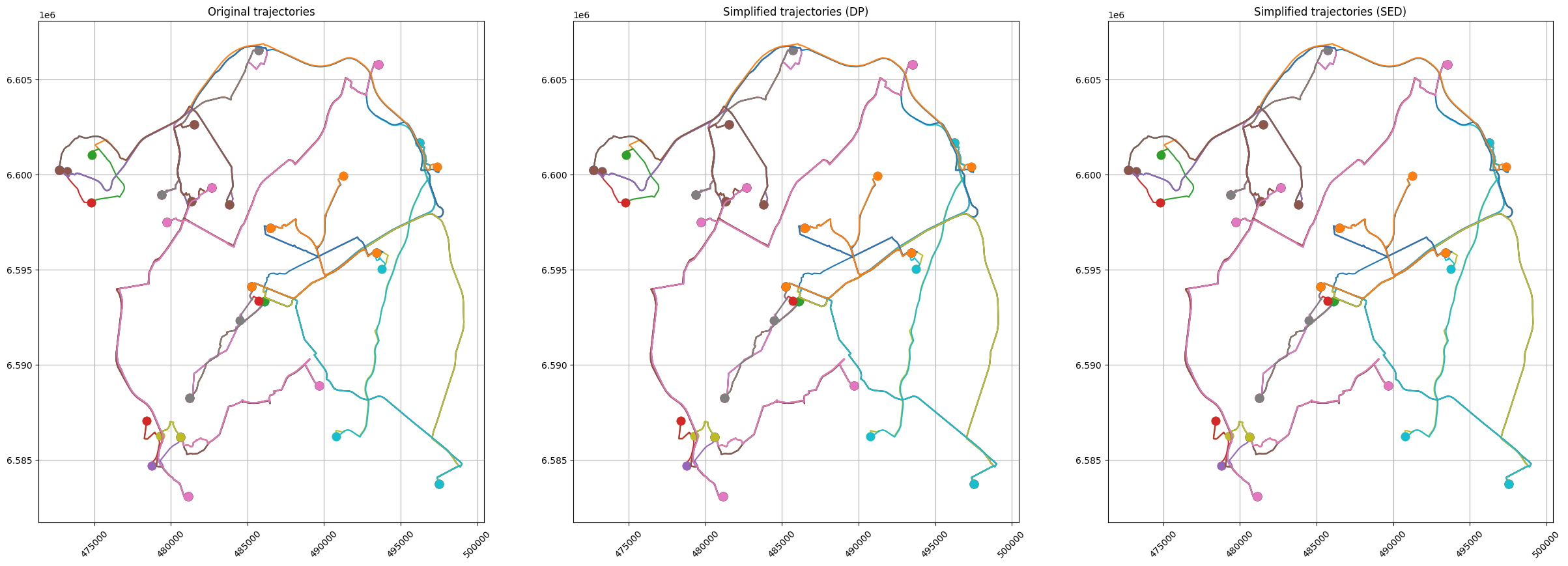
Simplifying Trips (MEOS Example)

In this section, we will simplify the trajectories with two different methods, namely Douglas-Peucker (DP) and Syncronized Euclidean Distance (SED, aka Top-Down Time Ratio simplification), and compare the simplifications.

First, we’ll choose a distance tolerance to use in the simplification

tolerance = 20

Now, we’ll compute both simplifications with the simplify_douglas_peucker method (using the synchronized parameter to chose between DP or SED)

simplifications = trips.copy()
simplifications["dp"] = simplifications["trip"].apply(
    lambda tr: tr.simplify_douglas_peucker(tolerance)
)
simplifications["sed"] = simplifications["trip"].apply(
    lambda tr: tr.simplify_douglas_peucker(tolerance, synchronized=True)
)
simplifications.head()

	vehicle	day	seq	trip	dp	sed
0	1	2020-06-01	1	[POINT(496253.84080706234 6601691.244869352)@2...	[POINT(496253.84080706234 6601691.244869352)@2...	[POINT(496253.84080706234 6601691.244869352)@2...
1	1	2020-06-01	2	[POINT(481241.17182724166 6588272.126511315)@2...	[POINT(481241.17182724166 6588272.126511315)@2...	[POINT(481241.17182724166 6588272.126511315)@2...
2	1	2020-06-02	1	[POINT(496253.84080706234 6601691.244869352)@2...	[POINT(496253.84080706234 6601691.244869352)@2...	[POINT(496253.84080706234 6601691.244869352)@2...
3	1	2020-06-02	2	[POINT(481241.17182724166 6588272.126511315)@2...	[POINT(481241.17182724166 6588272.126511315)@2...	[POINT(481241.17182724166 6588272.126511315)@2...
4	1	2020-06-03	1	[POINT(496253.84080706234 6601691.244869352)@2...	[POINT(496253.84080706234 6601691.244869352)@2...	[POINT(496253.84080706234 6601691.244869352)@2...

_, axes = plt.subplots(1, 3, figsize=(30, 10))
for _, trip in simplifications.iterrows():
    trip["trip"].plot(axes=axes[0])
    trip["dp"].plot(axes=axes[1])
    trip["sed"].plot(axes=axes[2])
axes[0].set_title("Original trajectories")
axes[1].set_title("Simplified trajectories (DP)")
axes[2].set_title("Simplified trajectories (SED)")
plt.show()

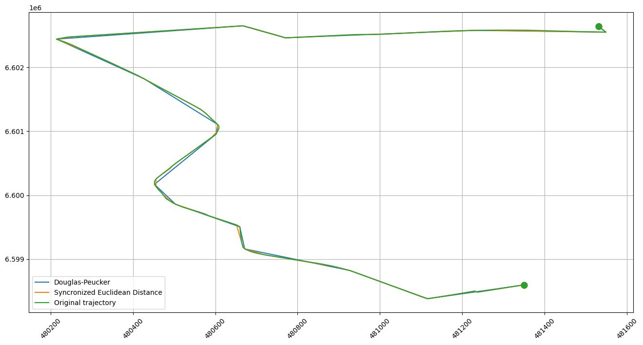
Let’s focus on only one trajectory to see the simplification more clearly

trip_example = simplifications.iloc[20]
fig, ax = plt.subplots(figsize=(16, 8))
trip_example["dp"].plot(label="Douglas-Peucker")
trip_example["sed"].plot(label="Syncronized Euclidean Distance")
trip_example["trip"].plot(label="Original trajectory")
plt.legend()
plt.savefig("./output.svg")

Now, let’s see the difference in points in each trajectory with their simplifications

distances = simplifications[["vehicle", "day", "seq"]].copy()
distances["trip"] = simplifications["trip"].apply(lambda tr: tr.num_instants())
distances["dp"] = simplifications["dp"].apply(lambda tr: tr.num_instants())
distances["sed"] = simplifications["sed"].apply(lambda tr: tr.num_instants())
distances["dp-delta"] = distances["trip"] - distances["dp"]
distances["sed-delta"] = distances["trip"] - distances["sed"]
distances["dp-%"] = distances["dp"] * 100 / distances["trip"]
distances["sed-%"] = distances["sed"] * 100 / distances["trip"]
distances.head()

	vehicle	day	seq	trip	dp	sed	dp-delta	sed-delta	dp-%	sed-%
0	1	2020-06-01	1	2103	48	212	2055	1891	2.282454	10.080837
1	1	2020-06-01	2	2326	65	232	2261	2094	2.794497	9.974205
2	1	2020-06-02	1	2110	48	207	2062	1903	2.274882	9.810427
3	1	2020-06-02	2	2308	65	235	2243	2073	2.816291	10.181976
4	1	2020-06-03	1	2071	48	190	2023	1881	2.317721	9.174312

We can see in the following table that the DP-simplified trips contain only a 3% of the original points in average, and that the SED-simplified ones around a 10%.

distances[["dp-delta", "dp-%", "sed-delta", "sed-%"]].describe()

	dp-delta	dp-%	sed-delta	sed-%
count	96.000000	96.000000	96.000000	96.000000
mean	1425.489583	2.686471	1315.750000	9.568915
std	718.930726	1.068704	649.342437	1.514393
min	98.000000	1.731844	91.000000	7.011070
25%	923.500000	1.999928	875.250000	8.475305
50%	1616.000000	2.367245	1471.500000	9.281897
75%	2056.750000	2.859347	1894.000000	10.622931
max	3333.000000	7.547170	2990.000000	14.150943

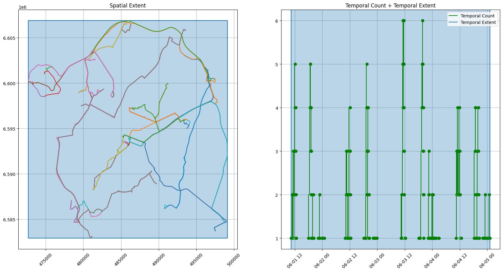
Temporal Aggregation of Trips (MEOS Example)

In this section we will aggregate the trips to calculate the extent (the spatiotemporal bounding box) and the temporal count (the evolution on time of the number of vehicles travelling). PyMEOS offers two APIs for aggregating: bulk and streaming.

Bulk aggregation

If you have all the elements to aggregate in memory, you can use the bulk aggregation to perform it in a single call. To do so, use the aggregate methods of the aggregator classes.

Now, let’s compute the extent and the temporal count using the TemporalPointExtentAggregator and TemporalPeriodCountAggregator respectively

extent_bulk = TemporalPointExtentAggregator.aggregate(trips["trip"])
tcount_bulk = TemporalPeriodCountAggregator.aggregate(trips["trip"])

_, axes = plt.subplots(1, 2, figsize=(20, 10))

extent_bulk.plot_xy(axes=axes[0], label="Spatial Extent")
for _, trip in trips.iterrows():
    trip["trip"].plot(axes=axes[0], show_markers=False)
axes[0].set_title("Spatial Extent")

tcount_bulk.plot(axes=axes[1], label="Temporal Count", color="g")
extent_bulk.to_tstzspan().plot(axes=axes[1], label="Temporal Extent")
axes[1].set_title("Temporal Count + Temporal Extent")

plt.legend()
plt.show()

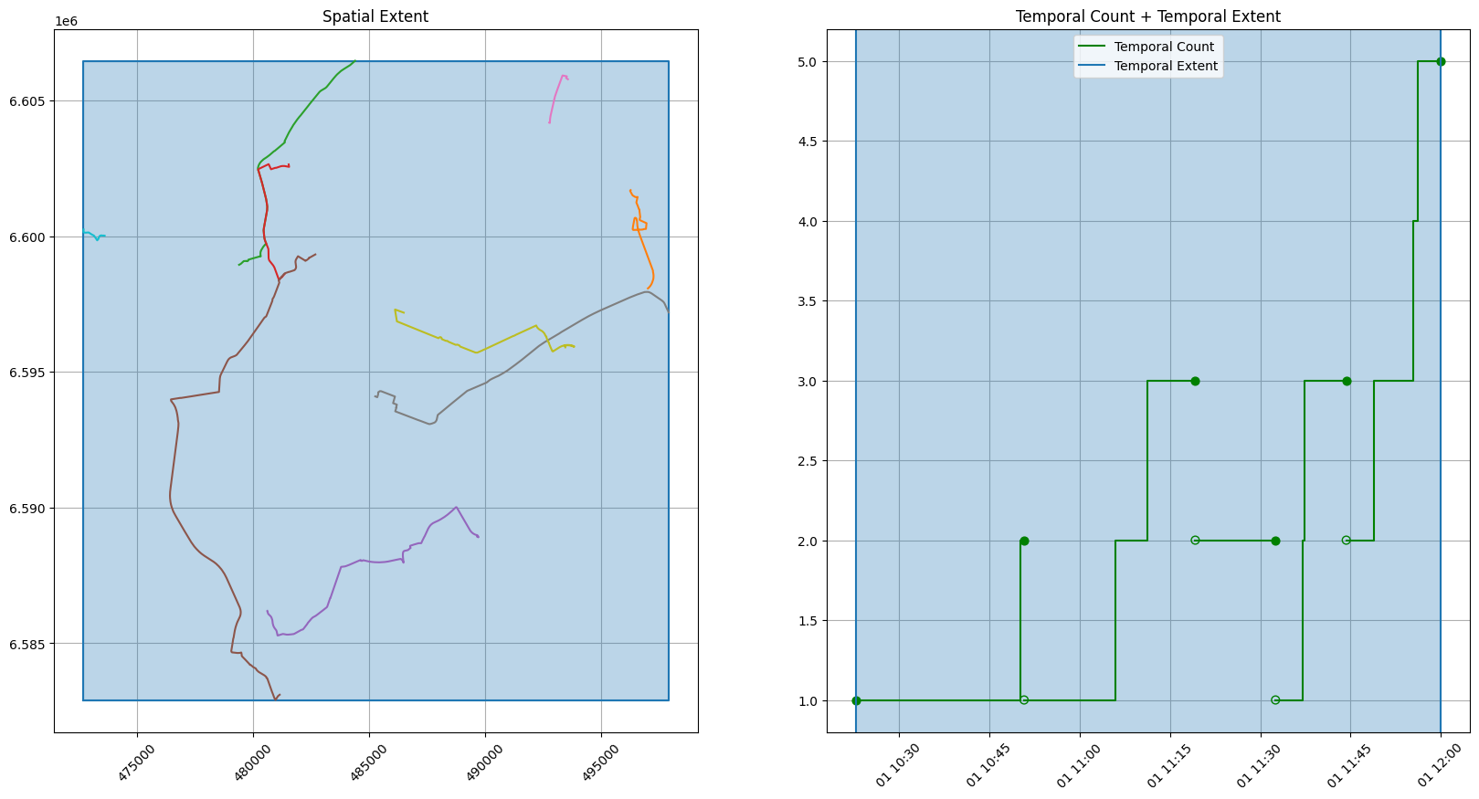
Let’s take the extent of only a few hours to see clearly the aggregations

day_trips = (
    trips["trip"]
    .apply(lambda tr: tr.at(TsTzSpan("[2020-06-01 08:00:00, 2020-06-01 12:00:00]")))
    .dropna()
)
day_extent = TemporalPointExtentAggregator.aggregate(day_trips)
day_tcount = TemporalPeriodCountAggregator.aggregate(day_trips)

_, axes = plt.subplots(1, 2, figsize=(20, 10))

day_extent.plot_xy(axes=axes[0], label="Spatial Extent")
for trip in day_trips:
    trip.plot(axes=axes[0], show_markers=False)
axes[0].set_title("Spatial Extent")

day_tcount.plot(axes=axes[1], label="Temporal Count", color="g")
day_extent.to_tstzspan().plot(axes=axes[1], label="Temporal Extent")
axes[1].set_title("Temporal Count + Temporal Extent")

plt.legend()
plt.show()

Streaming Aggregation

There will be cases when you don’t have all the elements in memory at once, for example, maybe there are too many and memory is limited, or you are receiving them on real time, and you want to aggregate as they arrive. In those cases, you can use the streaming aggregation to perform the aggregation in steps. To do so, use the start_aggregation method of the aggregator class, and then use the object returned to perform the aggregation using the add and aggregation methods.

extent_aggregator = TemporalPointExtentAggregator.start_aggregation()
count_aggregator = TemporalPeriodCountAggregator.start_aggregation()

for trip in trips["trip"]:
    extent_aggregator.add(trip)
    count_aggregator.add(trip)
extent_stream = extent_aggregator.aggregation()
count_stream = count_aggregator.aggregation()

_, axes = plt.subplots(1, 2, figsize=(20, 10))

extent_stream.plot_xy(axes=axes[0], label="Spatial Extent")
for _, trip in trips.iterrows():
    trip["trip"].plot(axes=axes[0], show_markers=False)
axes[0].set_title("Spatial Extent")

count_stream.plot(axes=axes[1], label="Temporal Count", color="g")
extent_stream.to_tstzspan().plot(axes=axes[1], label="Temporal Extent")
axes[1].set_title("Temporal Count + Temporal Extent")

plt.legend()
plt.show()

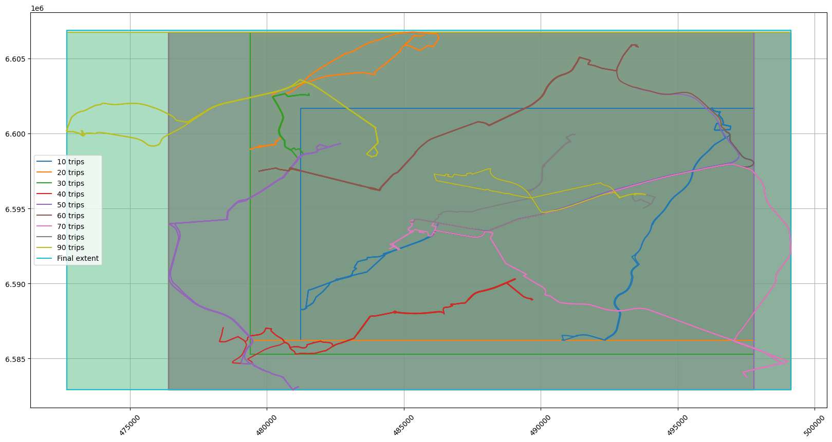
Note that you can keep aggregating after getting the result.

extent_aggregator = TemporalPointExtentAggregator.start_aggregation()
_, ax = plt.subplots(1, 1, figsize=(20, 10))
color = "black"
colors = []
for i, trip in enumerate(trips["trip"], 1):
    extent_aggregator.add(trip)
    if i % 10 == 0:
        plot = extent_aggregator.aggregation().plot_xy(label=f"{i} trips")
        color = plot[0][0].get_color()
        colors += [color] * 10
extent_stream = extent_aggregator.aggregation()
extent_stream.plot_xy(label="Final extent")

for trip, color in zip(trips["trip"], colors):
    trip.plot(show_markers=False, color=color)

plt.legend()
plt.show()

Tiling Trips (MEOS Example)

In this section, the trajectories and the speed will be split into tiles, for which we will compute some aggregates.

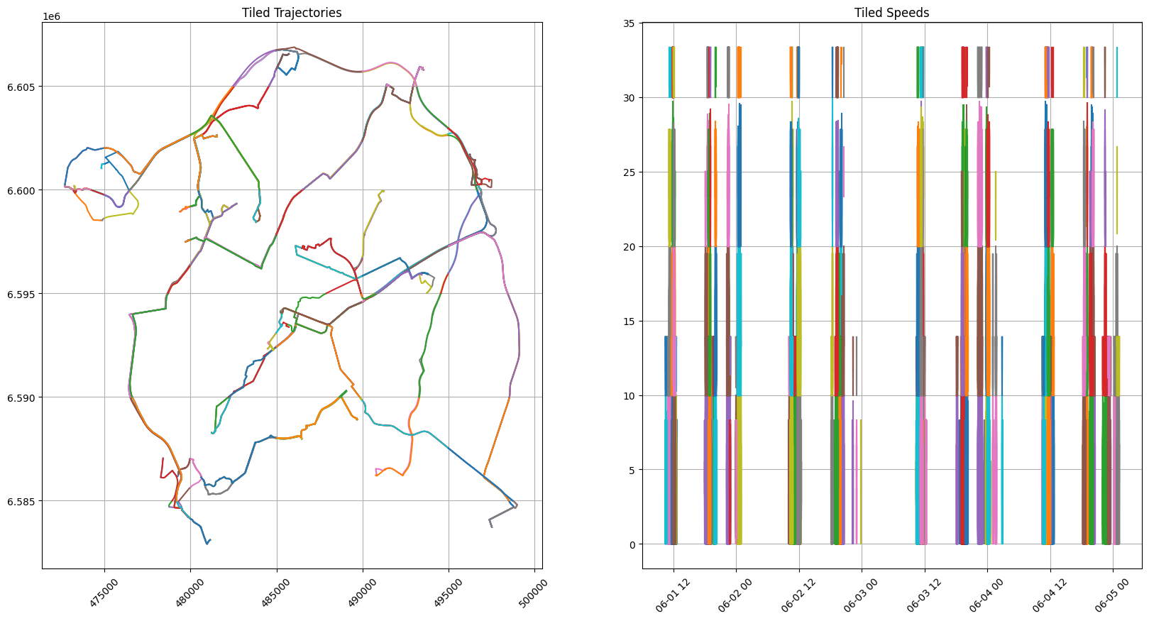
First, let’s take a look at the tiled trajectories and speeds

tiled_trips = trips["trip"].apply(lambda tr: tr.tile(5e3, remove_empty=True))
speeds = trips["trip"].apply(lambda tr: tr.speed())
tiled_speeds = speeds.apply(
    lambda sp: sp.value_time_split(10, "1 day", 0, "2020-06-01")
)

_, axes = plt.subplots(1, 2, figsize=(20, 10))
for tiled_trip in tiled_trips:
    for traj in tiled_trip:
        traj.plot(axes=axes[0], show_markers=False)
axes[0].set_title("Tiled Trajectories")

for tiled_speed in tiled_speeds:
    for traj in tiled_speed:
        traj.plot(axes=axes[1], show_markers=False)
axes[1].set_title("Tiled Speeds")

plt.show()

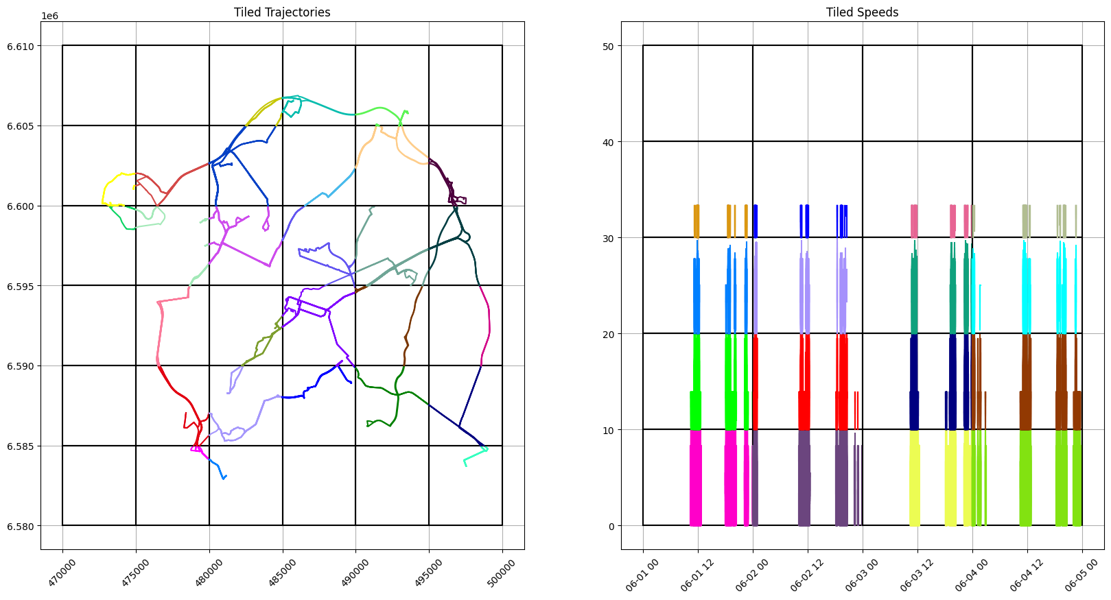
To see the tiles more clearly, let’s tile the extent of all the trips and speeds instead and compute the intersection of each trip with each tile (that is exactly what the tile function of TPointSeq is doing under the hood). This way, we can color them manually to see them clearly.

extent_tiles = extent_bulk.tile(5e3)
speed_extent = TemporalNumberExtentAggregator.aggregate(speeds)
speed_tiles = speed_extent.tile(10, "1 day", 0.0, "2020-06-01")

_, axes = plt.subplots(1, 2, figsize=(20, 10))

for tile, color in zip(extent_tiles, distinctipy.get_colors(len(extent_tiles))):
    tile.plot_xy(axes=axes[0], color="black", draw_filling=False)
    for trip in trips["trip"]:
        trip_in_tile = trip.at(tile)
        if trip_in_tile is not None:
            trip_in_tile.plot(axes=axes[0], color=color, show_markers=False)
axes[0].set_title("Tiled Trajectories")

for tile, color in zip(speed_tiles, distinctipy.get_colors(len(speed_tiles))):
    tile.plot(axes=axes[1], color="black", draw_filling=False)
    for speed in speeds:
        speed_in_tile = speed.at(tile)
        if speed_in_tile is not None:
            speed_in_tile.plot(axes=axes[1], color=color, show_markers=False)
axes[1].set_title("Tiled Speeds")
plt.show()

Finally, let’s aggregate the tiles to compute some metrics We will start by computing, for each spatial tile, the number of trajectories that enter it, and the total amount of time spent and the total distance traveled by them in the tile.

extent_tiles = extent_bulk.tile(5e3)
data = []
for tile in extent_tiles:
    intersections = trips["trip"].apply(lambda tr: tr.at(tile)).dropna()
    if len(intersections) == 0:
        continue
    count = len(intersections)
    duration = sum([i.duration() for i in intersections], timedelta())
    distance = sum([i.length() for i in intersections]) / 1000
    data.append([tile, count, duration, distance])

spatial_aggregates = pd.DataFrame(
    data, columns=["tile", "count", "duration", "distance"]
)

spatial_aggregates

	tile	count	duration	distance
0	SRID=3857;STBOX X((475000,6580000),(480000,658...	10	0 days 00:21:57.271928	12.715462
1	SRID=3857;STBOX X((480000,6580000),(485000,658...	8	0 days 00:37:50.260034	15.250435
2	SRID=3857;STBOX X((495000,6580000),(500000,658...	8	0 days 00:56:22.219006	19.807692
3	SRID=3857;STBOX X((475000,6585000),(480000,659...	13	0 days 01:42:26.592035	59.420951
4	SRID=3857;STBOX X((480000,6585000),(485000,659...	20	0 days 03:34:19.201837	73.582531
5	SRID=3857;STBOX X((485000,6585000),(490000,659...	12	0 days 02:07:10.468161	52.101740
6	SRID=3857;STBOX X((490000,6585000),(495000,659...	6	0 days 01:22:33.732748	36.422087
7	SRID=3857;STBOX X((495000,6585000),(500000,659...	8	0 days 00:47:50.956624	42.149632
8	SRID=3857;STBOX X((475000,6590000),(480000,659...	8	0 days 01:21:45.559201	54.962866
9	SRID=3857;STBOX X((480000,6590000),(485000,659...	10	0 days 01:39:18.880626	35.092058
10	SRID=3857;STBOX X((485000,6590000),(490000,659...	37	0 days 04:43:56.029545	135.629127
11	SRID=3857;STBOX X((490000,6590000),(495000,659...	21	0 days 01:08:30.026607	27.547398
12	SRID=3857;STBOX X((495000,6590000),(500000,659...	4	0 days 00:27:07.208503	20.924216
13	SRID=3857;STBOX X((470000,6595000),(475000,660...	9	0 days 00:16:51.436501	10.185846
14	SRID=3857;STBOX X((475000,6595000),(480000,660...	30	0 days 01:37:23.497930	38.060402
15	SRID=3857;STBOX X((480000,6595000),(485000,660...	40	0 days 05:02:47.976012	127.956860
16	SRID=3857;STBOX X((485000,6595000),(490000,660...	18	0 days 02:44:27.235479	69.741764
17	SRID=3857;STBOX X((490000,6595000),(495000,660...	28	0 days 03:01:46.069980	113.754468
18	SRID=3857;STBOX X((495000,6595000),(500000,660...	16	0 days 01:56:46.320943	79.532763
19	SRID=3857;STBOX X((470000,6600000),(475000,660...	14	0 days 01:08:43.444506	23.299969
20	SRID=3857;STBOX X((475000,6600000),(480000,660...	11	0 days 01:12:06.437047	55.651246
21	SRID=3857;STBOX X((480000,6600000),(485000,660...	26	0 days 04:36:55.024443	145.456576
22	SRID=3857;STBOX X((485000,6600000),(490000,660...	8	0 days 00:57:20.399942	36.388236
23	SRID=3857;STBOX X((490000,6600000),(495000,660...	12	0 days 01:54:33.371322	58.257905
24	SRID=3857;STBOX X((495000,6600000),(500000,660...	14	0 days 01:36:16.495602	46.346555
25	SRID=3857;STBOX X((480000,6605000),(485000,661...	10	0 days 00:40:21.652772	22.114868
26	SRID=3857;STBOX X((485000,6605000),(490000,661...	10	0 days 01:06:43.042539	33.102930
27	SRID=3857;STBOX X((490000,6605000),(495000,661...	12	0 days 00:41:57.630167	22.865846

For the speed tiles, we will compute the number of times a vehicle is in the speed range at that time, and the amount of time it stays there

speed_tiles = speed_extent.tile(10, "1 day", 0, "2020-06-01")
data = []
for tile in speed_tiles:
    intersections = speeds.apply(lambda tr: tr.at(tile)).dropna()
    if len(intersections) == 0:
        continue
    count = len(intersections)
    duration = sum([i.duration() for i in intersections], timedelta())
    data.append([tile, count, duration])

speed_aggregates = pd.DataFrame(data, columns=["tile", "count", "duration"])

speed_aggregates

	tile	count	duration
0	TBOXFLOAT XT([0, 10),[2020-06-01 00:00:00+02, ...	21	0 days 07:31:24.685901
1	TBOXFLOAT XT([10, 20),[2020-06-01 00:00:00+02,...	21	0 days 03:03:36.408255
2	TBOXFLOAT XT([20, 30),[2020-06-01 00:00:00+02,...	12	0 days 00:31:46.326571
3	TBOXFLOAT XT([30, 40),[2020-06-01 00:00:00+02,...	11	0 days 00:12:42.223983
4	TBOXFLOAT XT([0, 10),[2020-06-02 00:00:00+02, ...	23	0 days 07:39:36.356752
5	TBOXFLOAT XT([10, 20),[2020-06-02 00:00:00+02,...	21	0 days 03:02:29.137009
6	TBOXFLOAT XT([20, 30),[2020-06-02 00:00:00+02,...	12	0 days 00:31:04.548691
7	TBOXFLOAT XT([30, 40),[2020-06-02 00:00:00+02,...	11	0 days 00:14:00.514541
8	TBOXFLOAT XT([0, 10),[2020-06-03 00:00:00+02, ...	24	0 days 08:16:09.948028
9	TBOXFLOAT XT([10, 20),[2020-06-03 00:00:00+02,...	22	0 days 03:03:03.718551
10	TBOXFLOAT XT([20, 30),[2020-06-03 00:00:00+02,...	13	0 days 00:44:43.354712
11	TBOXFLOAT XT([30, 40),[2020-06-03 00:00:00+02,...	12	0 days 00:12:20.122468
12	TBOXFLOAT XT([0, 10),[2020-06-04 00:00:00+02, ...	28	0 days 09:01:32.980751
13	TBOXFLOAT XT([10, 20),[2020-06-04 00:00:00+02,...	26	0 days 03:23:41.826769
14	TBOXFLOAT XT([20, 30),[2020-06-04 00:00:00+02,...	14	0 days 00:38:43.298191
15	TBOXFLOAT XT([30, 40),[2020-06-04 00:00:00+02,...	12	0 days 00:10:49.332312